This post is part of my lecture notes on the theory of computation. This is lecture 1.

You can view all the articles under this serie here.

I decided to open source some of my university course notes instead of having them neatly packed in my google drive where they serve no purpose anymore. Consider them more of an addition to your primary materials.

I took this course from ADuni as a supplement to my university materials. There are many online video courses out there on all sorts of subjects but few impressed me like this one. It made a difficult subject easy and actually interesting!

Lecture 1

This course is about what things we can compute mechanically, how fast can we do it and how much space it requires. Practical applications of it:

• all of compiler design
• modelling a processor with a FSM
• string searching (FSM)
• XML which you describe with a grammar

For example we might want to compute the set of binary strings that end in zero, or the set that represents legal java programs (which a compiler can do).

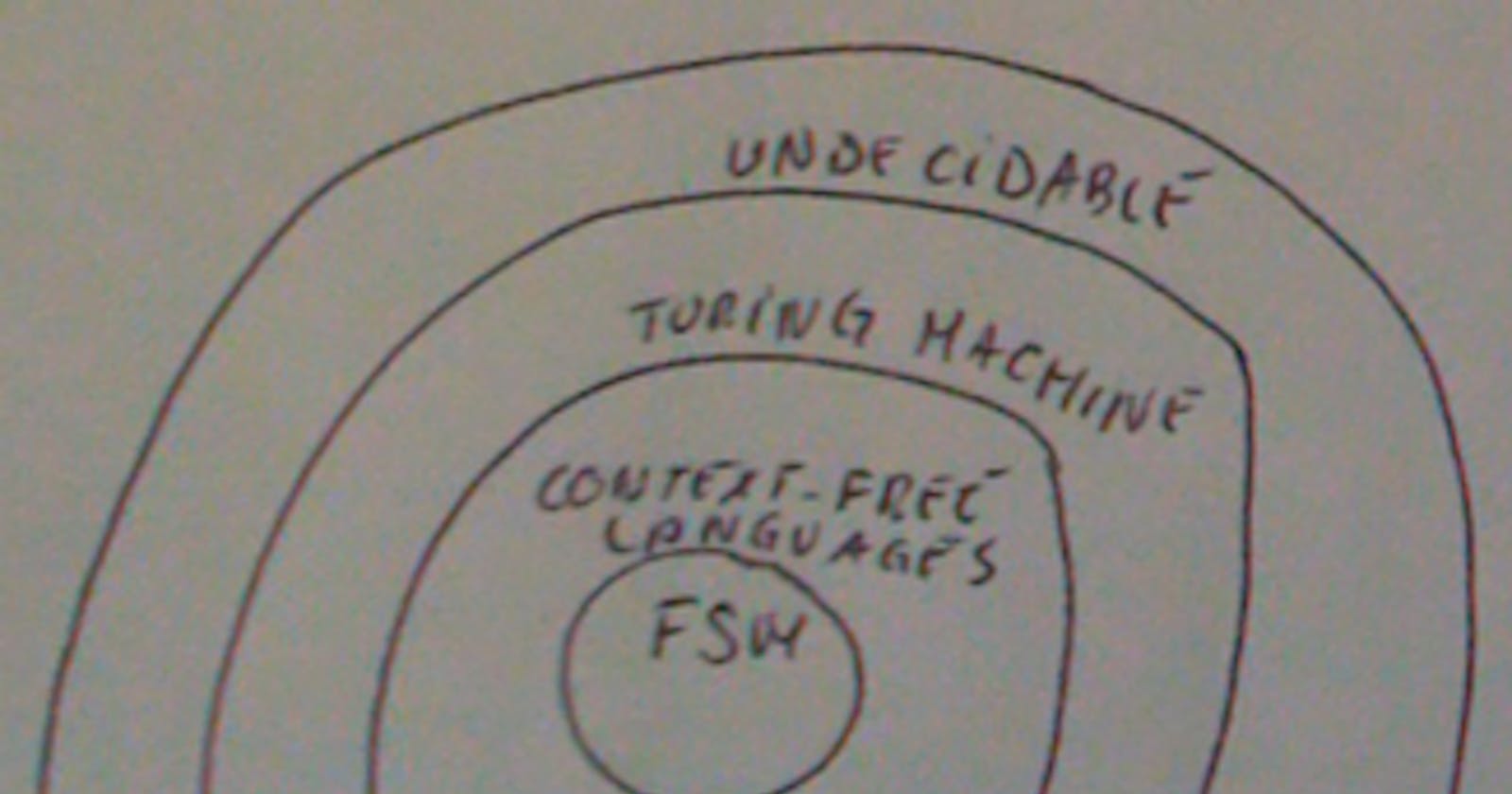
Turing machines are an abstract way to think about how programs are written and executed. Because of its simplicity and abstraction, we can use them to prove what programs can and cannot be written to work on a turning machine. The idea is that everything a normal PC can run (i.e. something a programming language can produce) a T.M. can also run.

We will work our way up to a TM starting from the finite state machine. This machine can do only certain kinds of sets and is much less powerful than a programming language.

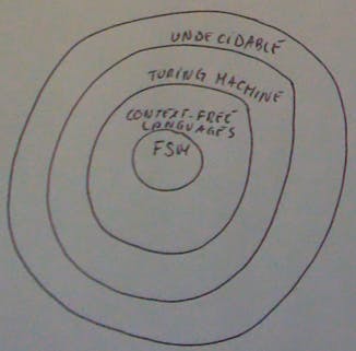
Inside this graph there are more details which for the present we will ignore (inside the TM there is another class called NP and inside that another one called P).

Finite state machine

A FSM has states which store information - they represent some kind of memory. An intuition for it: anything you can solve with a finite (i.e. constant) amount of memory, you can compute with a FSM.

We give each state a semantic meaning and we represent them using circles. Let’s start with an example: I want to find the binary strings that have an even number of zeros. A FSM that does that might look like this:

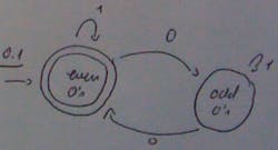
The double circle around the state indicates which state is to be the final state. Our FSM accepts all binary strings that have an even number of zeros and rejects those that don’t: if after the final bit we’re not in the final state. When we have a problem that we want to model using a FSM, before drawing the states we must think about how we want to model them.

Example: FSM for even number of zeros and even number of 1s. We have 4 states (first the 0 then the 1):

• even even (ee)
• even odd (eo)
• odd even (oe)
• odd odd (oo)

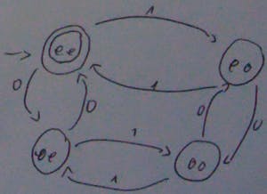
Note that we can have more than one final state. Ex: even number of 0 and 1 OR odd number of 0 and 1. Also note that the FSM from above works but it’s not the minimum FSM (we can in fact have only 2 states). There is an algorithm that does the minimisation - a dynamic programming algorithm.

Example: FSM for binary numbers divisible by 4. This means that we look at the last two numbers (4=2^2) to see if they are 0. Let’s first look at a FSM that checks if a binary string begins with 00 since it’s easier and then we’ll build on that.

Now to solve for strings that end with 00:

Note that we start from the final state (right side) and since we start from there we also accept empty strings. There is however, an easier way to do this: there is a way that we can easily find the FSM of a language for its reverse language, these are called closures and using them we can also find many other things. The reverse of things that are divisible by 4 are things that start with 00.

What about a FSM for numbers that aren’t divisible by 4? We can do this easily by reversing our FSM for numbers that are divisible by 4. We reverse the orders, the final state(s) become non-final and the others become final states. This is a type of closure. It’s said that FSMs are closed under complement; if you can do one kind of set, you can do its complement.

Example Write a FSM for 110110

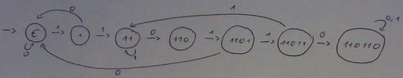
• the last state 110110 is the final state (forgot the double circle)

If we are at state 11011 and we get a 1, we don’t go all the way back but only to state 11.

It’s harder to focus on sets that don’t contain something; doing the opposite is easier - find the FSM for strings for a pattern - and then you find the closure.

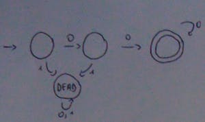
Example: every 1 is followed by at least two 0s.

In this figure you can see that there are two identical states (*).

The idea of minimising a FSM is to reduce states that do exactly the same thing. Below we have deleted the redundant state (the final state):

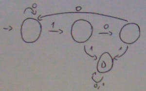
D stands for a dead state.

Example: binary strings that are not divisible by 3 (3 is not a power of 2 so can’t do the trick with zeros at the end).

Hint: Try to solve for numbers that are divisible by 3, then reverse it because it’s easier this way.

Problem: at each step we need to remember the result as we go along with the division and that size is proportional to the string and is not constant. Therefor the space required is not final (i.e. constant) -> we can’t do real division.

The way we do it is that we look at each number separately. If we have:

10111

1: the remainder of this first 1 div by 3 = 1.

0: adding a 0 to the end of our binary string doubles the number. We double the remainder which is now 2 (we try to divide the remainder by 3 and it's 2 so this is the result).

1: now again, we double the remainder and add 1. So 2*2=4 which is a remainder of 1 and adding 1 gives us 2.

And we continue this way; this is a recursive problem.

I’m keeping track of the remainder which can be one of these three: either 0, either 1 or either 2. We can model this FSM with just three states:

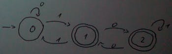
We have two final states.

Some things that you can’t do with finite state machines: counting, counting the number of zeros or ones in a number.

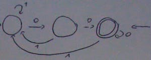
Non-deterministic FSM means that we can have more than one arrow with the same meaning (0 or 1 for example) coming out of the same state. Non-deterministic FSM are easier to write but they don’t add more power, in the sense that whatever we can write with a non-deterministic FSM we can write with a deterministic FSM. Taking our example from before which verifies that the string set is 110110.

Accepting a string in a non-deterministic FSM means that if there is a choice that will get you to a final state, then accept the string; otherwise if no choice gets you to a final state only then reject it. There can be many choices that don’t get you to the final state.

For example the string (we need to see if it has 110110):

11 110 110 11

needs to be accepted because a subset of it contains the string we’re searching for. Our non-deterministic FSM will look like this:

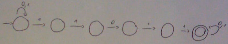
BTW note that a deterministic machine would reject this.

The set of choices that will get me to the final state are 1,1 the first state, then progress through the states with 110110, arrive at the final state and there do the last 0,0. Basically the states eats up the prefix strings until my string starts and eats the string at the end. There is no way to accept wrong strings since to arrive at the final state we need to have a 110110, there’s no other way to get there. The non-deterministic choices are at the front and back states in this case.

If I try to make the complement of the non-deterministic machine it won’t work as it was for deterministic machines because then my FSM will accept everything. The only way to get the complement is to convert it to deterministic and then complement it.

A computation for a ND FSM like in our case looks like a tree with each node having two children nodes:

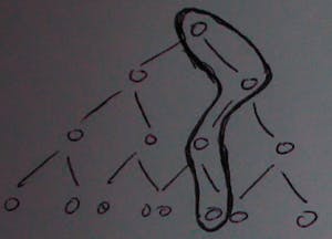
All the nodes represent parallel calculations, if there is a route to get to the final state you accept, if all the paths from the root don’t lead to the final state, you reject. A node might have only one other node if we then moves to a state which only accepts one input.

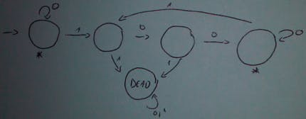
Now let’s try to create a ND FSM that accepts all the numbers which end in two zeroes. If there is no arrow telling me where to go then we don’t accept the string (or we can also explicitly add the dead states).

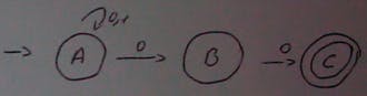
For the string 011001000 in the picture above, if we end up at the final state and have an extra zero we don’t accept, but there is a way that we can accept this string by arriving at the end with no extra zeros. Note that this machine doesn’t accept strings divisible by 4 because that would mean to accept a single 0 and empty strings which our ND FSM does not.

Now we convert this ND machine back to a deterministic machine using a mechanical process. At each step we write in what possible states the machine might be.

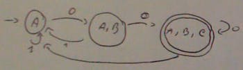
So for example with the string 0110 I can only be in A or B so I don’t accept it. I only accept if a string ends up in A, B, C because it has a chance to end up in C which is my final state. In our new deterministic machine the final states are all which include the final state from the ND machine.

Converting from a ND to a D machine in the worst case scenario I will see an exponential growth (2^n); in our example the number of states in the worst case could have been 2^3.